Setup here

An agents path through time, $t$ and space, $x = [x_1,x_2]$, denoted as space-time coordinates $q = [x_1,x_2, t]$, is represented by the curve $s$ . This curve is discretized by segments $e$. Each piece-wise constant rod segment encodes a scalar cost for the agent, which for now, is just kinetic energy, or $\frac{1}{2}mv^2$. The goal is to use CoV to find an optimal curve that maximizes total utility for the agent (minimizes kinetic energy over the path).

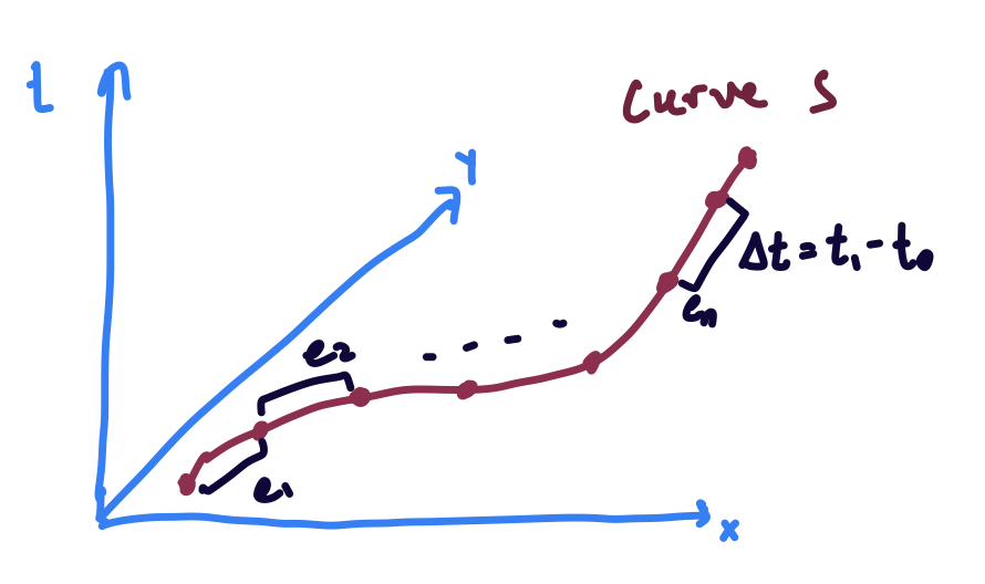
The discrete Lagrangian for each segment of the rod (just kinetic energy) can be written as

\[L = \frac{1}{2}m(\frac{x_1 - x_0}{t_1 - t_0})^2 \Delta t\]

where $m$ is the mass, $x_i$ and $t_i$ are the spatial and time coordinates of the two ends of the piece-wise constant segment. For each segment we can interpolate $q(s) = q_0 + s (q_1 - q_0)$. So, individually for space and time,

\[x = x_0 + s(x_1 - x_0) = x_0 + s\Delta x\]

and

\[t = t_0 + s(t_1 - t_0) = t_0 + s\Delta t\]

So, after discretizing the curve, hamilton’s principle of least action can be written as

\[S = \sum_{e=0}^{|e|-1} L(\Delta s, q_e, q_{e+1}) = \sum_{e=1}^{|e|-1} \frac{1}{2}m(\frac{x_{e+1} - x_e}{t_{e+1} - t_e})^2 (t_{e+1} - t_e)\tag{1}\]

Discrete CoV requires that the variation for the optimal rod be 0, so

\[\delta S = \delta \sum_{e=0}^{e = n-1} [D_2 L(\Delta s, q_e, q_{e+1})\cdot \delta q_e + D_3 L(\Delta s, q_e, q_{e+1})\cdot\delta q_{e+1}] = 0 \tag{2}\]

Boundary Conditions

After re-arranging and accounting for B.C.

\[\delta S = \delta \sum_{e=1}^{e = n-1} [D_3 L(\Delta s, q_{e-1}, q_e) + D_2 L(\Delta s, q_e, q_{e+1})]\cdot\delta q_{e} \\ + D_2 L(\Delta s, q_0, q_1)\cdot \delta q_0 + D_3 L(\Delta s, q_{n -1}, q_{n})\cdot \delta q_{n} = 0 \tag{3}\]

Since, we don’t want to fix the endpoint of the curve in time (only in space), our boundary condition is a bit funny, $\delta t_{n} = unknown$, which means that $D_3 L(\Delta s, q_{n -1}, q_n) = 0$ wrt $t_n$.

So we get the regular boundary conditions $\delta q_0 = 0$ (since it is known), $\delta x_n = 0$ (since its known), and finally, since $\delta t_n = ?$,

\[\frac{-m (x_{n} - x_{n-1})^2}{2(t_{n} - t_{n -1})^2} = 0\]

which means that the agent should stop by $t_n$.

Minimizing the functional

Since variation $\delta S = 0$ at the optimal function, we know the gradients

\[D_3 L(\Delta s, q_{e-1}, q_e) + D_2 L(\Delta s, q_e, q_{e+1}) = \frac{\partial L(\Delta s, q_{e-1}, q_e)}{\partial q_e} + \frac{\partial L(\Delta s, q_e, q_{e+1})}{\partial q_e} = 0\]

are zero. This will need to be done component-wise, since $q = [x, t]$.

\[\frac{\partial L(\Delta s, q_{e-1}, q_e)}{\partial q_e} + \frac{\partial L(\Delta s, q_e, q_{e+1})}{\partial q_e} = [\frac{\partial L(\Delta s, q_{e-1}, q_e)}{\partial x_e}, \frac{\partial L(\Delta s, q_{e-1}, q_e)}{\partial t_e}] + [\frac{\partial L(\Delta s, q_e, q_{e+1})}{\partial x_e}, \frac{\partial L(\Delta s, q_e, q_{e+1})}{\partial t_e}]\]

then

\[[\frac{m(x_e - x_{e-1})}{t_e - t_{e-1}}, \frac{m(x_e - x_{e-1})^2}{2(t_e - t_{e-1})^2}] + [\frac{-m(x_{e+1} - x_e)}{t_{e+1} - t_e}, \frac{-m(x_{e+1} - x_e)^2}{2(t_{e+1} - t_{e})^2}] = 0\]

so

\[[\frac{m(x_e - x_{e-1})}{t_e - t_{e-1}}, \frac{m(x_e - x_{e-1})^2}{2(t_e - t_{e-1})^2}] = [\frac{m(x_{e+1} - x_e)}{t_{e+1} - t_e}, \frac{m(x_{e+1} - x_e)^2}{2(t_{e+1} - t_{e})^2}]\]

which means that the kinetically optimal path for the agent is to have constant velocity until it reaches the end position. Which makes sense.