Abstract

To be written.

Intro

The idea is that agent paths through space and time can be denoted by a 3D curve where time is the z-axis and the x-y plane is the ground. For any given $t$, the projection of the curve onto the x-y plane gives the spatial coordinates of the agent at that $t$. Since each agent has a size, mass, and other physical characteristics, we use elastic rods with different characteristics extruded along the space-time curve to represent agent paths. Large agents are represented by large rod radiuses, and so on… Resolving collisions on these rods provides us with a collision-free trajectories for agents in the scene.

Related Works

Game Theory / Econ / Equilibrium

• Papadimitrou, Roughgarden - Polynomial Time Corr. Equilibrium for many different types of games
• Aumann - Correlated Equlibrium for N-player games

Crowds

• Trueille 2006 - Continuum Crowds
• Kapadia 2015 - book
• Pelechano 2016 - overview of several approaches, social dynamics
• Karamazous 2018 - comparing different algorithms
• Narain 2009 - continuum based approach, high densities
• Karamazous 2017 - implicit crowds, large timesteps, stable
• Hughes 2008 - vision based crowds
• Boids 1987
• Golas 2013 - Long range collision avoidance. Gradient based.
• Holden 2017 - Data driven approach to motion
• Lerner 2007 - Data driven
• Terzopolous 2018 - PBD crowds
• Warp Driver 2016 - vision based
• Van De Berg 2011 - collision free velocity updates through geometry

Space-time optimization

• Reconfigurables 2017 - detecting and modifying colliding geometries using space-time methods
• Witkin space-time constraints -
• Popovic ? Cant find this
• Barbic - Deformable object animation using reduced optimal control
• Popovic - Interactive Manipulation of Rigid Body

Collisions

• Barnes Hut
• Li 2020 - Incremental Potential Contact

Method

Our central assumption is that agents will choose a path which optimizes a utility function. This utility function could include a number of different metrics such as the total distance traveled, distance to obstacles, distance from other agents etc… The infinite number of paths available to an agent will each correspond to a single utility value. However, this injective mapping from path to utility is insufficient since agents also move through time. Therefore we introduce a third dimension for time and the notion of a space-time curve which denotes agent paths through time. Now, each space-time curve corresponds to a single utility. Our objective is to maximize agent utility by finding the optimal path through time.

We use discrete calculus of variations to find the optimal curve through space time. Our problem is similar to the derivation for the Euler-Lagrange equations, however in our case, the end boundary condition is not fixed in time; our agents are merely bounded by a max time. This is also the main difference between our method and previous space-time constraint papers (like Witkin et al) which have fixed time intervals and a fixed endpoint. Trying to solve for the optimal curve in space-time using continuous calculus of variations without having a fixed end time leads to very complex and incomprehensible second order differential equations, with strange boundary conditions. However, in the discrete CoV case, we get intuitive results.

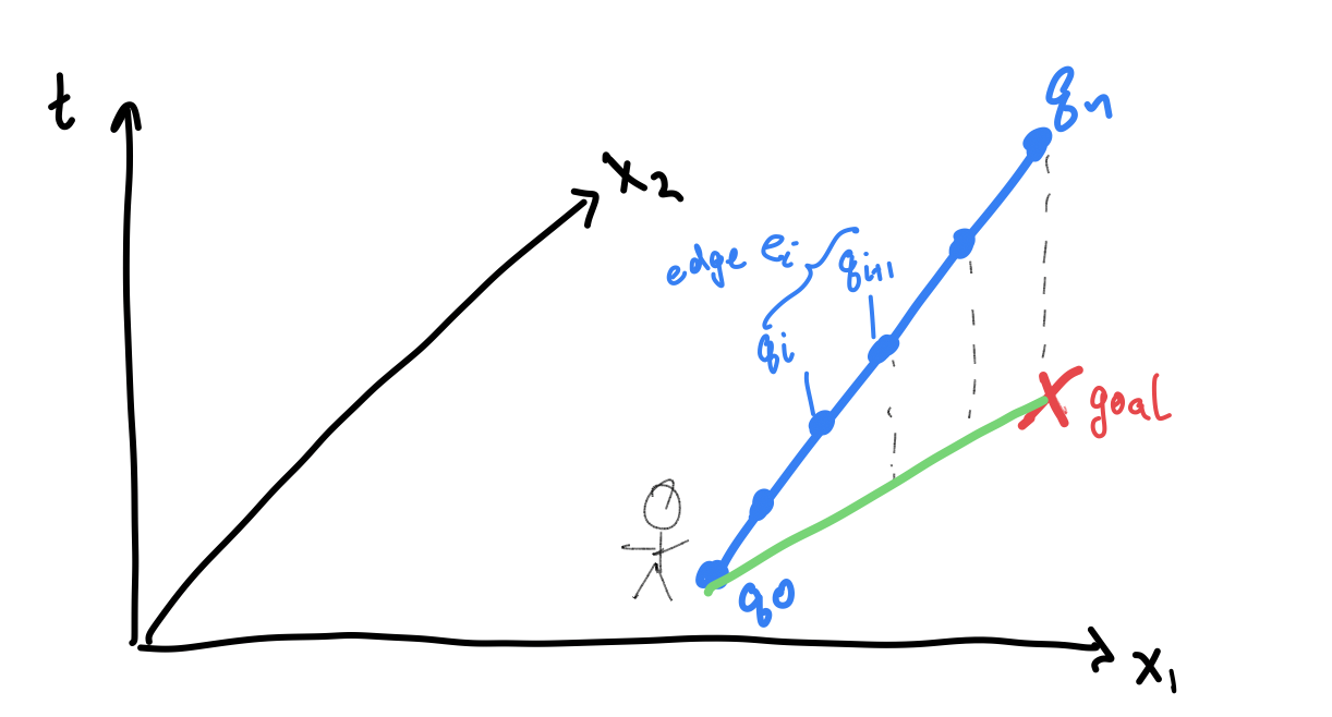
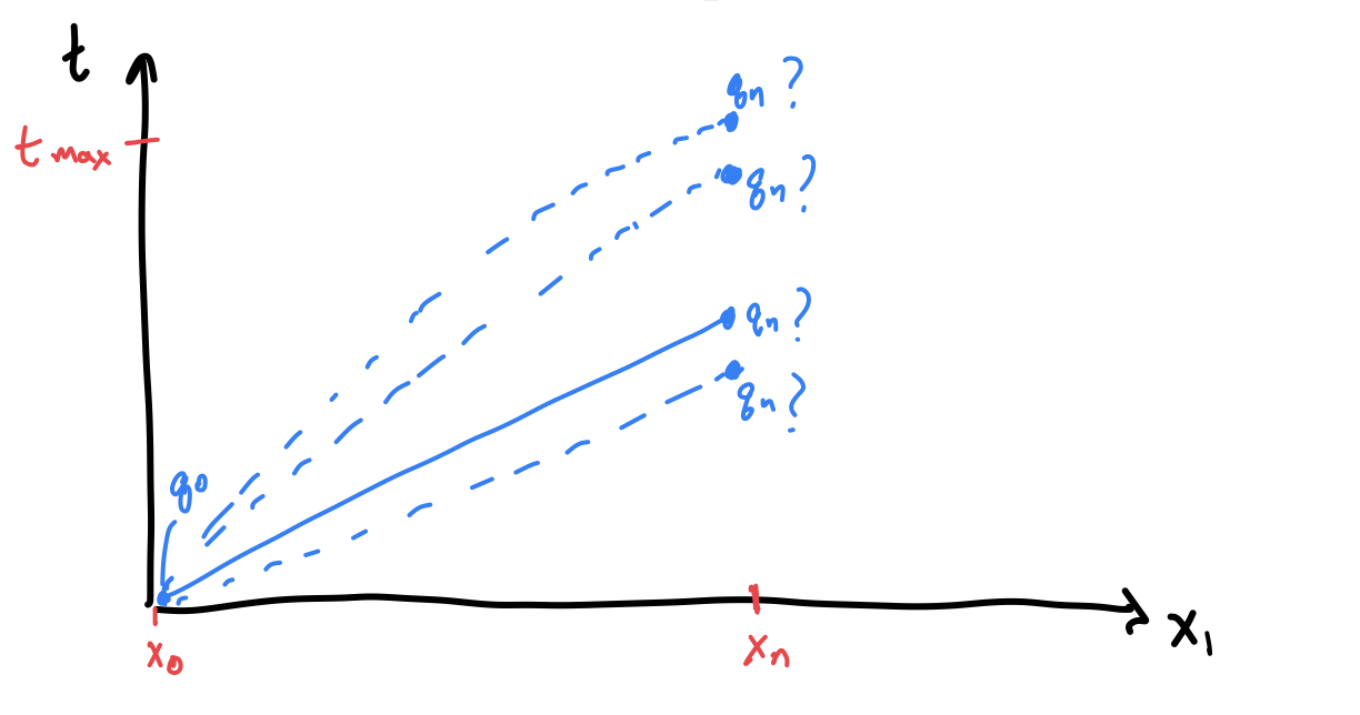
The first step is to discretize the space-time curves into $i=0..n$ vertices where each vertex $q_i = [x_i, t_i]$ describes the agent’s 2D position on ground $x_i$ and in time $t_i$. Each edge $e_i$ connects two adjacent vertices $q_i, q_i+1$.

The simplest utility function requires agents to minimize their kinetic energy expended in reaching their destination. The discrete Lagrangian for each segment of the rod (just kinetic energy) can be written as

\[L = \frac{1}{2}m(\frac{x_1 - x_0}{t_1 - t_0})^2 \Delta t\]

where $m$ is the mass, $x_i$ and $t_i$ are the spatial and time coordinates of the two ends of the piece-wise constant segment. For each segment we can interpolate $q(s) = q_0 + s (q_1 - q_0)$. So, individually for space and time,

\[x = x_0 + s(x_1 - x_0) = x_0 + s\Delta x\]

and

\[t = t_0 + s(t_1 - t_0) = t_0 + s\Delta t\]

So, after discretizing the curve, hamilton’s principle of least action can be written as

\[S = \sum_{e=0}^{|e|-1} L(\Delta s, q_e, q_{e+1}) = \sum_{e=1}^{|e|-1} \frac{1}{2}m(\frac{x_{e+1} - x_e}{t_{e+1} - t_e})^2 (t_{e+1} - t_e)\tag{1}\]

Discrete CoV requires that the variation for the optimal rod be 0, so

\[\delta S = \delta \sum_{e=0}^{e = n-1} [D_2 L(\Delta s, q_e, q_{e+1})\cdot \delta q_e + D_3 L(\Delta s, q_e, q_{e+1})\cdot\delta q_{e+1}] = 0 \tag{2}\]

Boundary Conditions

After re-arranging and accounting for B.C.

\[\delta S = \delta \sum_{e=1}^{e = n-1} [D_3 L(\Delta s, q_{e-1}, q_e) + D_2 L(\Delta s, q_e, q_{e+1})]\cdot\delta q_{e} \\ + D_2 L(\Delta s, q_0, q_1)\cdot \delta q_0 + D_3 L(\Delta s, q_{n -1}, q_{n})\cdot \delta q_{n} = 0 \tag{3}\]

Since, we don’t want to fix the endpoint of the curve in time (only in space), our boundary condition is a bit funny, $\delta t_{n} = unknown$, which means that $D_3 L(\Delta s, q_{n -1}, q_n) = 0$ wrt $t_n$.

So we get the regular boundary conditions $\delta q_0 = 0$ (since it is known), $\delta x_n = 0$ (since its known), and finally, since $\delta t_n = unkown$,

\[\frac{-m (x_{n} - x_{n-1})^2}{2(t_{n} - t_{n -1})^2} = 0\]

which means that the agent should stop by $t_n$.

Minimizing the functional

Since variation $\delta S = 0$ at the optimal function, we know the gradients

\[D_3 L(\Delta s, q_{e-1}, q_e) + D_2 L(\Delta s, q_e, q_{e+1}) = \frac{\partial L(\Delta s, q_{e-1}, q_e)}{\partial q_e} + \frac{\partial L(\Delta s, q_e, q_{e+1})}{\partial q_e} = 0\]

are zero. This will need to be done component-wise, since $q = [x, t]$.

\[\frac{\partial L(\Delta s, q_{e-1}, q_e)}{\partial q_e} + \frac{\partial L(\Delta s, q_e, q_{e+1})}{\partial q_e} = [\frac{\partial L(\Delta s, q_{e-1}, q_e)}{\partial x_e}, \frac{\partial L(\Delta s, q_{e-1}, q_e)}{\partial t_e}] + [\frac{\partial L(\Delta s, q_e, q_{e+1})}{\partial x_e}, \frac{\partial L(\Delta s, q_e, q_{e+1})}{\partial t_e}]\]

then

\[[\frac{m(x_e - x_{e-1})}{t_e - t_{e-1}}, \frac{m(x_e - x_{e-1})^2}{2(t_e - t_{e-1})^2}] + [\frac{-m(x_{e+1} - x_e)}{t_{e+1} - t_e}, \frac{-m(x_{e+1} - x_e)^2}{2(t_{e+1} - t_{e})^2}] = 0\]

so

\[[\frac{m(x_e - x_{e-1})}{t_e - t_{e-1}}, \frac{m(x_e - x_{e-1})^2}{2(t_e - t_{e-1})^2}] = [\frac{m(x_{e+1} - x_e)}{t_{e+1} - t_e}, \frac{m(x_{e+1} - x_e)^2}{2(t_{e+1} - t_{e})^2}]\]

which means that the kinetically optimal path for the agent is to have constant velocity until it reaches the end position. Which makes sense since it indicates the agent’s momentum is constant along the path which indicates that net forces acting on the agent along the path are 0.

In Practice

The CoV derivations for the optimal space-time rod indicate that the optimal can be found by simply minimizing the kinetic energy along the rod with a few additional constraints. The equality constraints are the start and end positions of the agent. The inequality constraints are that $t_n \leq T_{max}$ and time monotonically increases $t_i \leq t_{i+1}$. In the simplest case of one agent, the optimization can be written as follows:

\[min_q \; E(q) \\ s.t.\\ q_0 = [X_0, T_0] \\ x_n = X_n \\ t_n \leq T_{max} \\ t_i \leq t_{i+1}\]

where the capitals $X_0, T_0, X_n, T_{max}$ are boundary conditions. This energy, currently, is just kinetic energy.

With two or more agents on intersecting paths, $q$ generalizes to all the agents. A simple collision resolution constrain is added to prevent rod intersections, which results in the following equation

\[min_q \; E(q = [q_1, q_2]) \\ s.t.\\ q_0 = [X_0, T_0] \\ x_n = X_n \\ t_n \leq T_{max} \\ t_i \leq t_{i+1} \\ AllPointsDistance(q_1, q_2) \geq tolerance\]