Yale Financial Markets Lecture 3

In equilibrium, the final allocation maximizes total welfare:

\[\sum_i W_i(x,m) = u_i(x) + m\]

Where $W_i$ is welfare of agent $i$ and $u_i(x)$ is the utility of agent $i$ for the quantity $x$, and $m$ is the utility of money.

Example with 2 agents

With two different goods $x, y$.

Agent A: Welfare: $W^A(x, y) = 100x - \frac{1}{2}x^2 + y$ Endowment: $e^A = (e^A_x, e^A_y) = (4, 5000)$

Agent B: Welfare: $W^B(x, y) = 30x - \frac{1}{2}x^2 + y$ Endowment: $e^B = (e^B_x, e^B_y) = (80, 1000)$

What is the equilibrium that maximizes utility?

• Exogenous variables: Welfare, endowments

• Endogenous variables:

  • $P_x, P_y, x^A, y^A, x^B, y^B$
  • $P_x, P_y$ are prices
  • This is what gets decided during the equilibrium computation.

Optimization Equations

$Max_{x,y}$ $W^A(x,y)$ s.t. $P_x x + P_y y <= P_x 4 + P_y 5000$

$Max_{x,y}$ $W^B(x,y)$ s.t. $P_x x + P_y y <= P_x 80 + P_y 1000$

The amount of goods equals the amount of endowments of the two agents. \(x^A + x^B = e^A_x + e^B_x = 80 + 4 = 84 \tag{1}\) \(y^A + y^B = e^A_y + e^B_y = 6000 \tag{2}\)

Since both agents are optimizing, they won’t waste money, so the $<=$ becomes and equality. \(P_x x^A + P_y y^A = 4P_x + 5000 P_y \tag{3}\) \(P_x x^B + P_y y^B = 80P_x + 1000 P_y \tag{4}\)

The marginal utility equations below show the value at which each agent is indifferent.

\[\frac{MU^A_x(x^A, y^A)}{P_x} = \frac{\frac{\partial W^A}{\partial x}}{P_x} = \frac{100 -x^A}{P_x} = \frac{MU^A_y(x^A, y^A)}{P_y} = \frac{\frac{\partial W^A}{\partial y}}{P_y} = \frac{1}{P_y} \tag{5}\] \[\frac{MU^B_x(x^B, y^B)}{P_x} = \frac{\frac{\partial W^B}{\partial x}}{P_x} = \frac{30 -x^B}{P_x} = \frac{MU^B_y(x^B, y^B)}{P_y} = \frac{\frac{\partial W^B}{\partial y}}{P_y} = \frac{1}{P_y} \tag{6}\]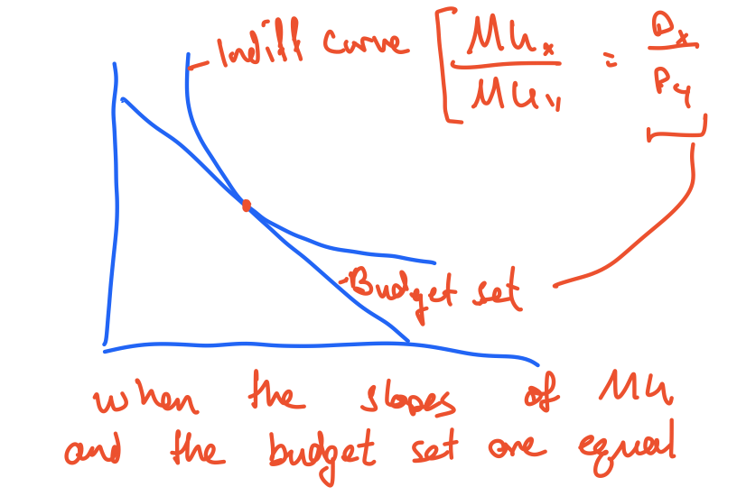

Arrow/Debreu/Mckenzie: This system of economics equations always has a solution. Based on Nash equilibrium and diminishing marginal utility.

Ok lets solve it now:

Walras 1871: Doubling the prices won’t change the equilibrium. The only thing that matters is relative prices.

Start with 6 eq, 6 unknowns:

Assume $P_y =1$.

Assume equations 1,3,4,5,6 are all satisfied. Then equation 2 has to be satisfied since everyone, collectively is spending all their money.

Now 5 eq, 5 unknowns:

Fix $P_y =1$. Then by eq 5, $\frac{100-x^B}{P_x} = 1$, so $x^A = 100-P_x$.

And by eq 6, $\frac{30-x^B}{P_x} = 1$, so $x^B = 30 - P_x$

Now since $x^A + x^B = 84$ then $P_x = 23$. Therefore $x^A = 77$ and $x^B = 7$.

Plug these into eq 3,4 to figure out $y^A, y^B$.

Another example with 2 agents

Cobb-Douglas Utility Function: Each person spends a fixed proportion of their money on each of the goods. Sum of logs.

Agent C:

• Welfare: $W^C(x, y) = \frac{3}{4}log(x) + \frac{1}{2}log(y)$
• Endowment: $e^C = (e^C_x, e^C_y) = (2, 1)$

Agent D:

• Welfare: $W^D(x, y) = \frac{2}{3}log(x) + \frac{1}{3}log(y)$
• Endowment: $e^C = (e^C_x, e^C_y) = (1, 2)$

Equations

Supply/Demand:

\[x^C + x^D = e^C_x + e^D_x = 2 + 1 = 3 \tag{1}\] \[y^C + y^D = e^C_y + e^D_y = 1 + 2 = 3 \tag{2}\]

Budget Set:

\[P_x x^C + P_y y^C = 2P_x + Py \tag{3}\] \[P_x x^D + P_y y^D = P_x + 2Py \tag{4}\]

Marginal Utility:

\[\frac{MU_x(x^C, y^C)}{P_x} = \frac{\frac{3}{4}\frac{1}{x^C}}{P_x} = \frac{\frac{1}{4}\frac{1}{y^C}}{P_y} = \frac{MU_x(x^C, y^C)}{P_y} \tag{5}\] \[\frac{MU_x(x^D, y^D)}{P_x} = \frac{\frac{2}{3}\frac{1}{x^D}}{P_x} = \frac{\frac{1}{3}\frac{1}{y^D}}{P_y} = \frac{MU_x(x^D, y^D)}{P_y} \tag{5}\]

Solve this now

1. Assume $P_y = 1$. Solve eq. 5 for $x^C $.

2. $\frac{3}{4} \frac{1}{P_x x^C} = \frac{1}{4} \frac{1}{P_y y^C}$.
   • So person C will spend $\frac{3}{4}$ on $x$ and $\frac{1}{4}$ on $y$.
   • Similarly, person D will spend $\frac{2}{3}$ on $x$ and $\frac{1}{3}$ on $y$.
3. The amount of money person C spends on $x$ is 3/4 of his income. And Person D is 2/3 of income
   • $P_x x^C = \frac{3}{4}[2P_x + P_y]$
   • $P_x x^D = \frac{2}{3}[2P_x + P_y]$
   • Since $P_y = 1$, then $x^C + x^D = 3$ Solving these equations, we get $P_x = \frac{5}{2}$, $x^C = \frac{9}{5}$ and $x^D = \frac{6}{5}$

Solving the linear system

These problems are solveable through least square minimization of a linear system $Ax = b$

Unknowns are $(P_x, P_y, x^C, x^D, y^C, y^D)$. Equations and constraints are encoded into lhs $A$ and the rhs $b$.